Practicals on SCZ GWAS 2022
Overview
In this practicals, we are going to analyze the GWAS from Schizophrenia 2022 to showcase how to use the new modules from FUMA v2.0.0
Download and Format GWAS
Download the GWAS summary statistics for the Schizophrenia GWAS from 2022 (https://pubmed.ncbi.nlm.nih.gov/35396580/) from https://pgc.unc.edu/for-researchers/download-results/
Download the file PGC3_SCZ_wave3.european.autosome.public.v3.vcf.tsv.gz
Tip
ALWAYS inspect the GWAS summary statistics file and format it before submitting to FUMA
Use zless PGC3_SCZ_wave3.european.autosome.public.v3.vcf.tsv.gz to view the content of the file. You will see that the file contains many lines with the # symbol before the actual data:
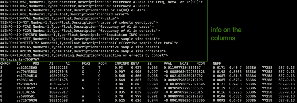
Check which build, GRCh37 or GRCh38
- Spot check a few variants on gnomad, the chromosome and position matches with GRCh37. For example:
Check which alleles are reference vs alternate
From the image above, it says A1 is the SNP reference allele and A2 is the SNP alternate allele. This matches with the information from gnomad as well.
Check other columns
p value is found under column name PVAL
beta is found under column name BETA
Sample sizes: there are 3 columns for sample size in this file: NCAS, NCON, and NEFF. For this practicals, I will define the sample size as equal to the sum of NCAS and NCON.
FCAS and FCON are the frequency of A1 in cases and controls, respectively.
Let’s prepare the input GWAS sumstat for running SNP2GENE and FLAMES.
For simplicity, I will prepare the input GWAS sumstat for running FLAMES, which I will also use for running a standard SNP2GENE analysis
Follow the instruction in https://fuma-docs.readthedocs.io/en/latest/flames/quick_start.html#submit-a-snp2gene-job
Based on the instruction, I will subset the file PGC3_SCZ_wave3.european.autosome.public.v3.vcf.tsv.gz to contain the following columns: CHROM, ID, POS, A1, A2, BETA, and PVAL. Example codes:
import gzip

outfile = open("scz2022_sumstat_fuma.txt", "w")

with gzip.open("PGC3_SCZ_wave3.european.autosome.public.v3.vcf.tsv.gz", "rt") as f:
    for line in f:
        if line.startswith("#"):
            continue
        fields = line.strip().split("\t")
        chrom = fields[0]
        pos = fields[2]
        id = fields[1]
        a1 = fields[3]
        a2 = fields[4]
        beta = fields[8]
        pval = fields[10]
        print("\t".join([chrom, id, pos, a1, a2, beta, pval]), file=outfile)
Run FLAMES
In this section we will try to identify the effect genes by running FLAMES
Step 1. Run SNP2GENE with MAGMA
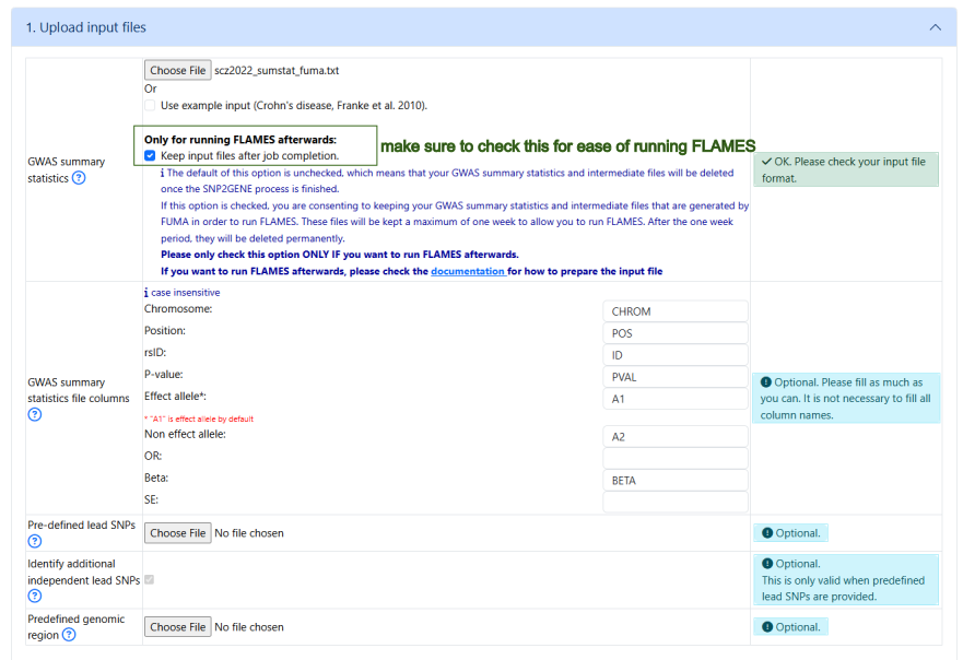
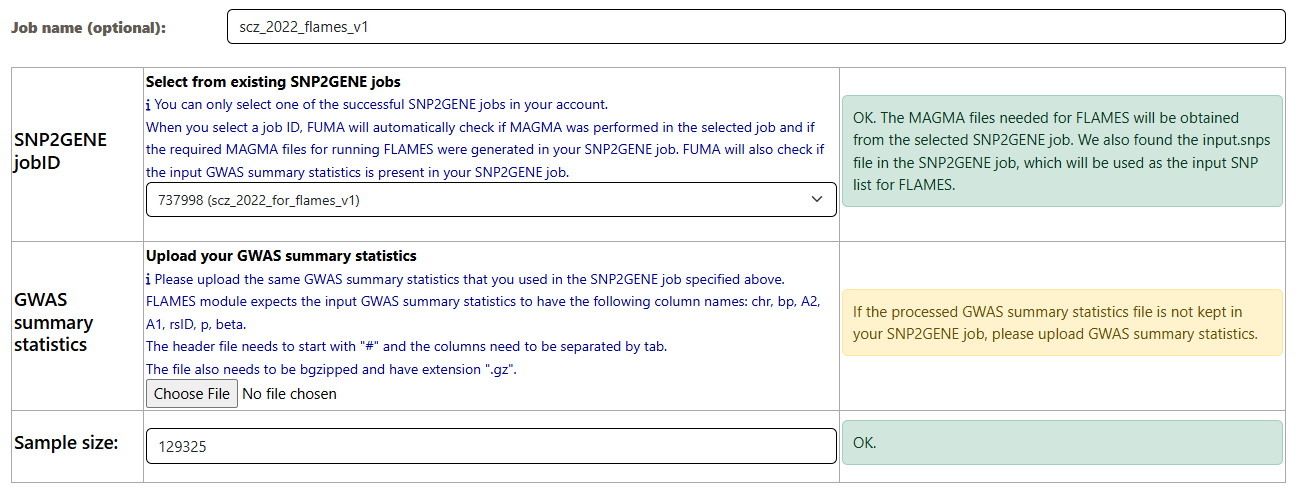
Submit a SNP2GENE job
Make sure to click on the button to keep the input gwas sumstat file for easy implementation of FLAMES
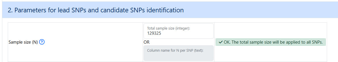
Make sure to put in an integer value for the sample size
Section 3-5 can be left as default
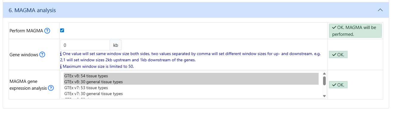
Make sure to check MAGMA in section 6
Put in a title and submit

Job finished successfully:

Step 2. Submit a FLAMES job
Run a SNP2GENE job with xQTLs mapping
In this section we will run a SNP2GENE job with xQTLs mapping
In theory, you can combine this with the run for FLAMES. However, it could be the case that MAGMA take a long time. Because each job has a limit of 8 hours, I recommend to run the MAGMA job separately.
Step 1. Submit a SNP2GENE job
Make sure to leave the button to keep the input gwas sumstat file UNCHECKED (this is the default)
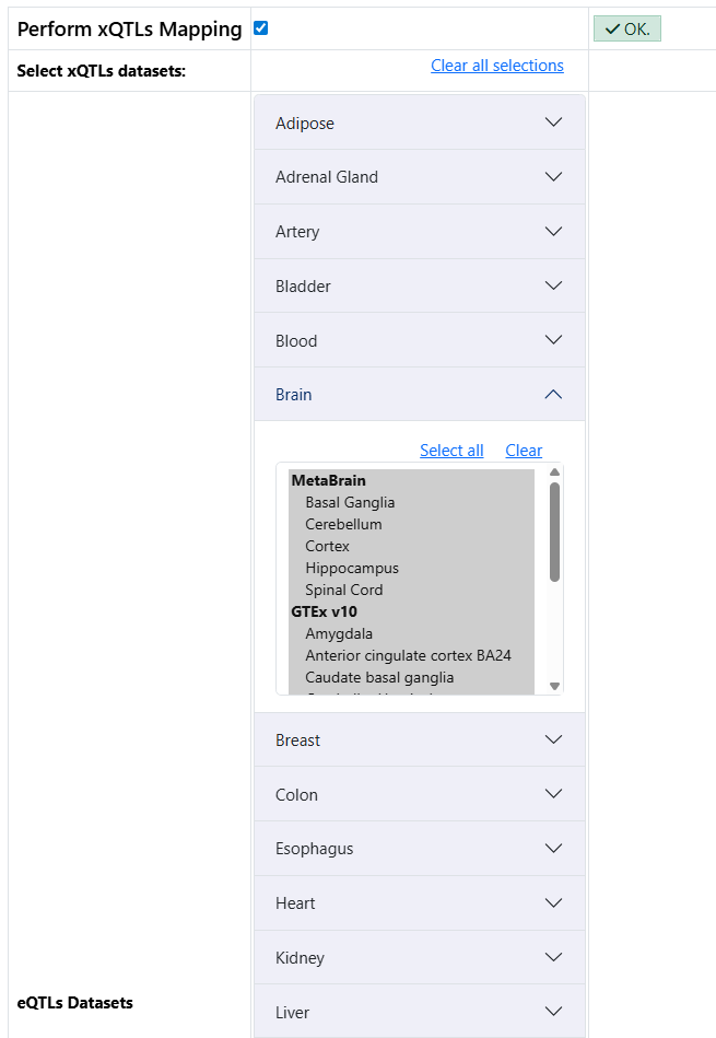
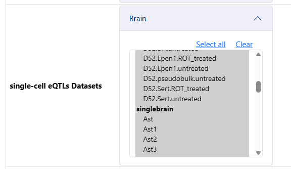
- In step 3, click on Perform xQTLs Mapping to expand the options and select the datasets
- Because I know apriori that schizophrenia is a brain related phenotype, I will select brain related xQTLs datasets
eQTLs from the brain
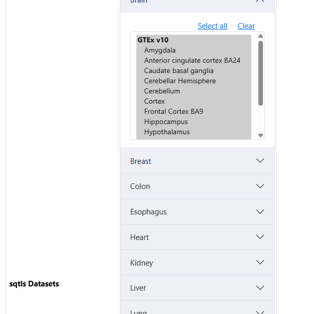
sQTLs from the brain
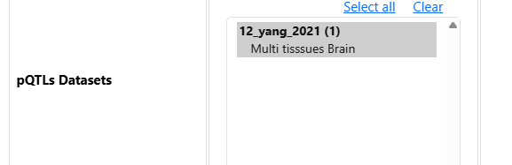
pQTLs from the brain
sceQTLs from the brain
Analysis: Find predicted relevant genes per genomic risk locus
- In this section, we are going to perform follow-up analyses after:
running a SNP2GENE job to map genes using positional mapping and xQTLs mapping
running a FLAMES job which predicts an effector gene per genomic risk locus
- We are interested in: which genes are predicted as being relevant for our GWAS when using:
positional mapping
xQTLs mapping
FLAMES
1. Download the result files from SNP2GENE - Download Gene table (mapped genes) and xQTLs mapping results
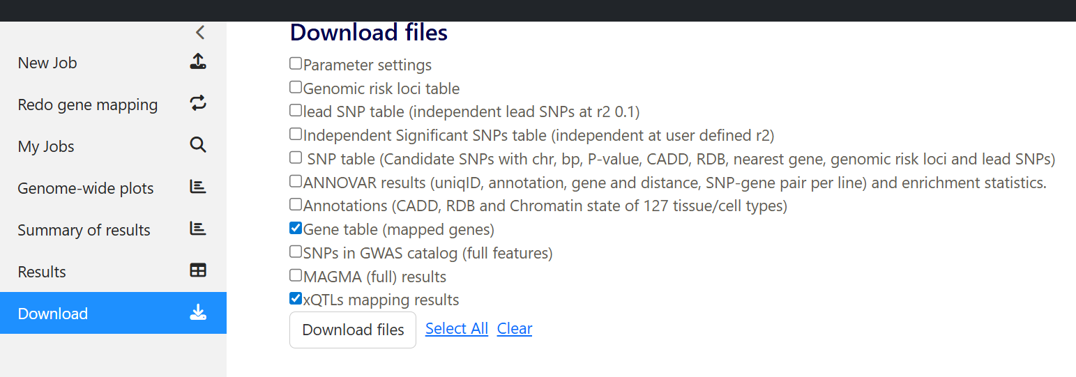
Then, unzip the folder
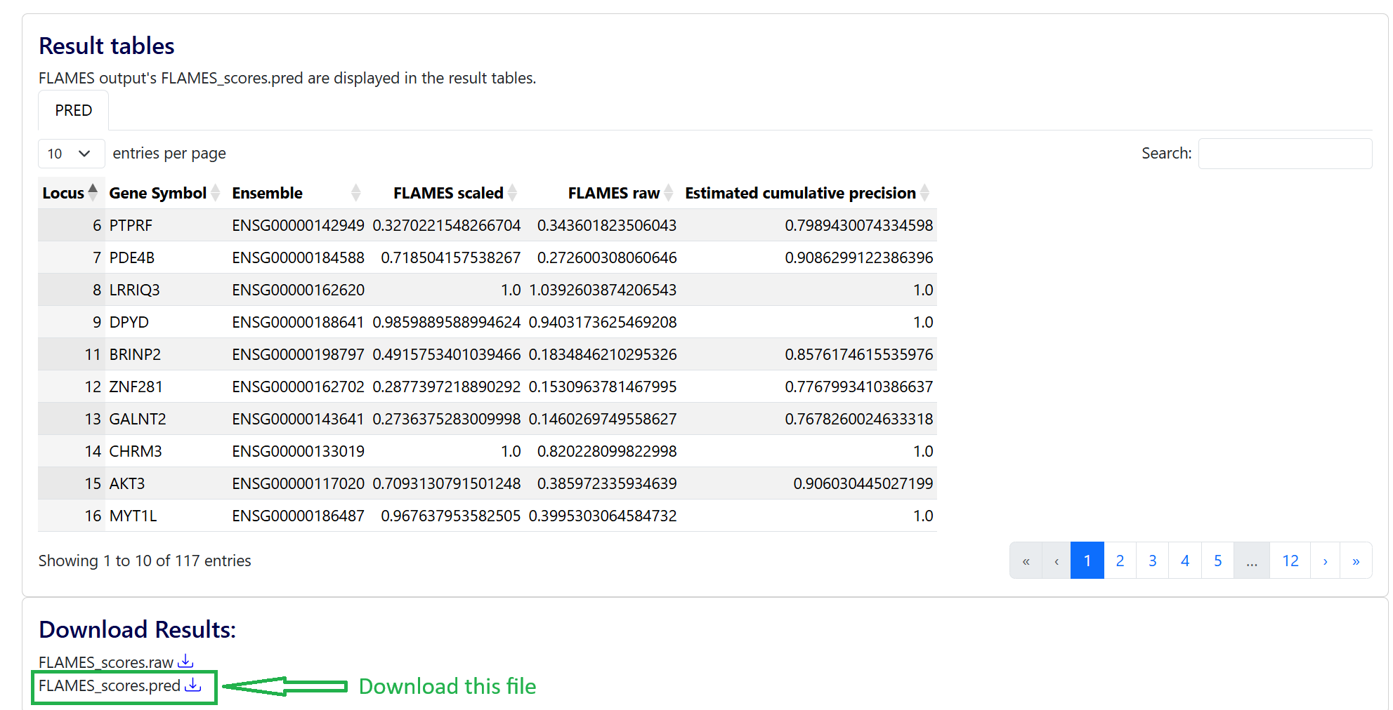
Download the result file from FLAMES
Create a directory called scz_2022 and copy and renames these files
mv genes.txt scz_2022/positional_mapped_genes.txt
mv mv xqtls.txt scz_2022/xqtls_mapped_genes.txt
mv FLAMES_scores_fmt.pred scz_2022/flames_mapped_genes.txt
Then, run script list_predicted_genes_per_locus.py (available at: https://github.com/tanyaphung/commonly_used_codes/tree/master/fuma_related/list_predicted_genes)
python list_predicted_genes_per_locus.py --filedir scz_2022/
- The above script returns:
column 1: genomic risk locus
column 2: whether it is positional (for positional mapping), xqtls (for xqtls mapping), or flames
column 3: the predicted or relevant gene
column 4: only in the xqtls mapping, it returns the name of the datasets
Tip
Analyze each genomic risk locus one at a time
Example from genomic risk locus 6
3 genes were mapped using positional mapping:
awk -F "," '$1==6{print}' mapped_genes.txt | grep positional
6,positional,PTPRF,
6,positional,KDM4A,
6,positional,ST3GAL3,
18 genes where the GWAS hits were also xQTLs:
awk -F "," '$1==6{print}' mapped_genes.txt | grep xqtls | awk -F "," '{print$3}' | sort | uniq
ARTN
ATP6V0B
CCDC24
CDC20
DPH2
ERI3
FAM183A
HYI
IPO13
KDM4A
MED8
PPIH
PTPRF
ST3GAL3
SZT2
TIE1
TMEM125
YBX1
FLAMES predicted PTPRF to be the effector gene
awk -F "," '$1==6{print}' mapped_genes.txt | grep flames
6,flames,PTPRF,
We then can run an QTLs Analysis module on FUMA to gain additional insights on the effects of GWAS variants within genomic risk locus 6
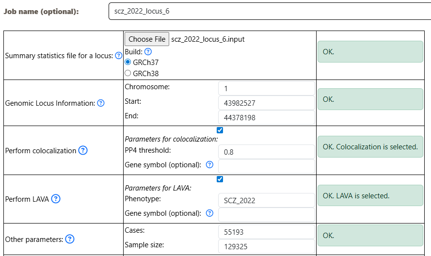
Example running QTLs Analysis
1. Obtain the range for genomic risk locus 6 - You can obtain this from the Results table, under tab Genomic risk loci:
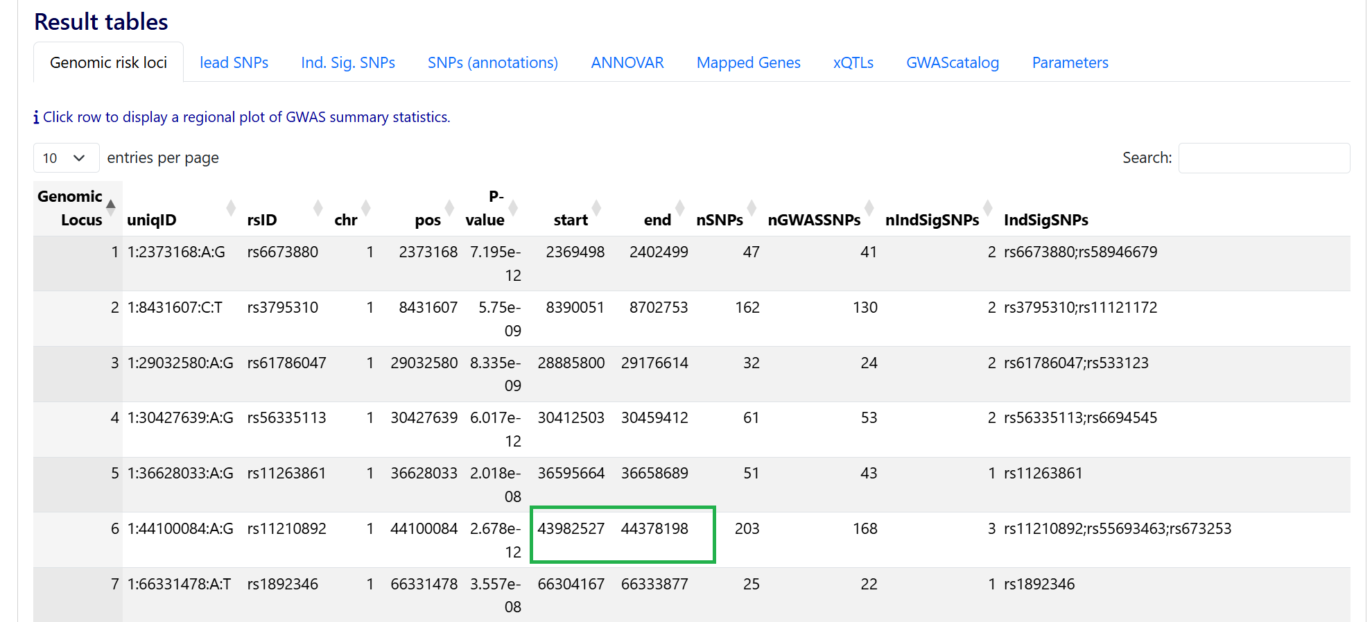
the range is chr1:43982527-44378198
2. Subset the GWAS sumstat for this range - For illustration purpose, let’s use FCON as the MAF - Example code:
import gzip

outfile = open("scz2022_sumstat_fuma.txt", "w")

with gzip.open("PGC3_SCZ_wave3.european.autosome.public.v3.vcf.tsv.gz", "rt") as f:
    for line in f:
        if line.startswith("#"):
            continue
        fields = line.strip().split("\t")
        chrom = fields[0]
        pos = fields[2]
        id = fields[1]
        a1 = fields[3]
        a2 = fields[4]
        beta = fields[8]
        pval = fields[10]
        print("\t".join([chrom, id, pos, a1, a2, beta, pval]), file=outfile)
3. Submit a QTLs Analysis job for genomic risk locus 6 - We can use the results from the xQTLs mapping to inform our selection of datasets. For example:
eQTL:gtex_v10:Brain_Cerebellar_Hemisphere
eQTL:gtex_v10:Brain_Cerebellum
eQTL:gtex_v10:Brain_Cortex
eQTL:gtex_v10:Brain_Frontal_Cortex_BA9
eQTL:metabrain:Brain_cerebellum
eQTL:metabrain:Brain_cortex
sceQTL:brainscope:Brain_brainscope_L2.3.IT
sceQTL:bryois2022Brain:Brain_bryois2022Brain_Astrocytes
sceQTL:bryois2022Brain:Brain_bryois2022Brain_Endothelial.cells
sceQTL:bryois2022Brain:Brain_bryois2022Brain_Excitatory.neurons
sceQTL:bryois2022Brain:Brain_bryois2022Brain_OPCs
sceQTL:jerber2021Dopaminergic:Brain_jerber2021Dopaminergic_D11.FPP
sceQTL:jerber2021Dopaminergic:Brain_jerber2021Dopaminergic_D11.P_FPP
sceQTL:jerber2021Dopaminergic:Brain_jerber2021Dopaminergic_D30.DA
sceQTL:jerber2021Dopaminergic:Brain_jerber2021Dopaminergic_D30.Epen1
sceQTL:jerber2021Dopaminergic:Brain_jerber2021Dopaminergic_D30.FPP
sceQTL:jerber2021Dopaminergic:Brain_jerber2021Dopaminergic_D30.Sert
sceQTL:jerber2021Dopaminergic:Brain_jerber2021Dopaminergic_D52.Epen1.ROT_treated
sceQTL:jerber2021Dopaminergic:Brain_jerber2021Dopaminergic_D52.Epen1.untreated
sceQTL:jerber2021Dopaminergic:Brain_jerber2021Dopaminergic_D52.Sert.ROT_treated
sceQTL:jerber2021Dopaminergic:Brain_jerber2021Dopaminergic_D52.Sert.untreated
sceQTL:jerber2021Dopaminergic:Brain_jerber2021Dopaminergic_D52.pseudobulk.untreated
sceQTL:singlebrain:Brain_singlebrain_Ast
sceQTL:singlebrain:Brain_singlebrain_Ext3
sceQTL:singlebrain:Brain_singlebrain_Ext5
sceQTL:singlebrain:Brain_singlebrain_Ext7
sceQTL:singlebrain:Brain_singlebrain_MG2
sceQTL:singlebrain:Brain_singlebrain_MiGA3
Note that the datasets from single brain can only be implemented with LAVA currently.
Submit a QTLs Analysis job:
- width:
800